Degrees of Freedom

Building an Intuition for Understanding Degrees of Freedom

Introduction

Degrees of freedom (df) is one of the most confusing concepts in statistics, yet it’s fundamental to understanding statistical inference.

What Are Degrees of Freedom?

Degrees of freedom represent the number of independent pieces of information available to estimate a parameter or test a hypothesis. Think of it as the number of “free choices” you have after accounting for constraints.

Vector Examples

---

The Intuition: The “Free to Vary” Concept

Simple Example: Three Numbers That Sum to 10

Let’s start with a simple example to build intuition:

# Check and install required packages
required_packages <- c("ggplot2", "dplyr")

# Load required packages
library(ggplot2)
library(dplyr)



# Install and load packages


# Set seed for reproducibility
set.seed(123)

# Example: Three numbers that sum to 10
cat("Constraint: x + y + z = 10\n\n")

Constraint: x + y + z = 10

# If we know two numbers, the third is determined
x <- 3
y <- 4
z <- 10 - x - y  # z is NOT free to vary

cat("If x =", x, "and y =", y, "then z MUST be", z, "\n")

If x = 3 and y = 4 then z MUST be 3 

cat("Degrees of freedom = 2 (only x and y are free to vary)\n")

Degrees of freedom = 2 (only x and y are free to vary)

Visualizing the Constraint

# Create a 2D visualization of the constraint x + y + z = 10
# We'll show how z is determined by x and y

# Generate points on the constraint plane
x_vals <- seq(0, 10, length.out = 50)
y_vals <- seq(0, 10, length.out = 50)

# Create grid of x and y values
grid_data <- expand.grid(x = x_vals, y = y_vals)
grid_data$z <- 10 - grid_data$x - grid_data$y

# Filter valid points (all coordinates >= 0)
valid_points <- grid_data[grid_data$z >= 0, ]

# Create 2D plot showing the constraint
ggplot(valid_points, aes(x = x, y = y, color = z)) +
  geom_point(size = 1, alpha = 0.6) +
  scale_color_gradient(low = "blue", high = "red", name = "z value") +
  labs(title = "Constraint: x + y + z = 10",
       subtitle = "Color shows the z value (red = high, blue = low)",
       x = "x value", y = "y value") +
  theme_minimal() +
  theme(plot.title = element_text(hjust = 0.5),
        plot.subtitle = element_text(hjust = 0.5)) +
  geom_abline(intercept = 10, slope = -1, color = "black", linewidth = 1, linetype = "dashed") +
  annotate("text", x = 8, y = 1, label = "x + y = 10", color = "black", size = 4)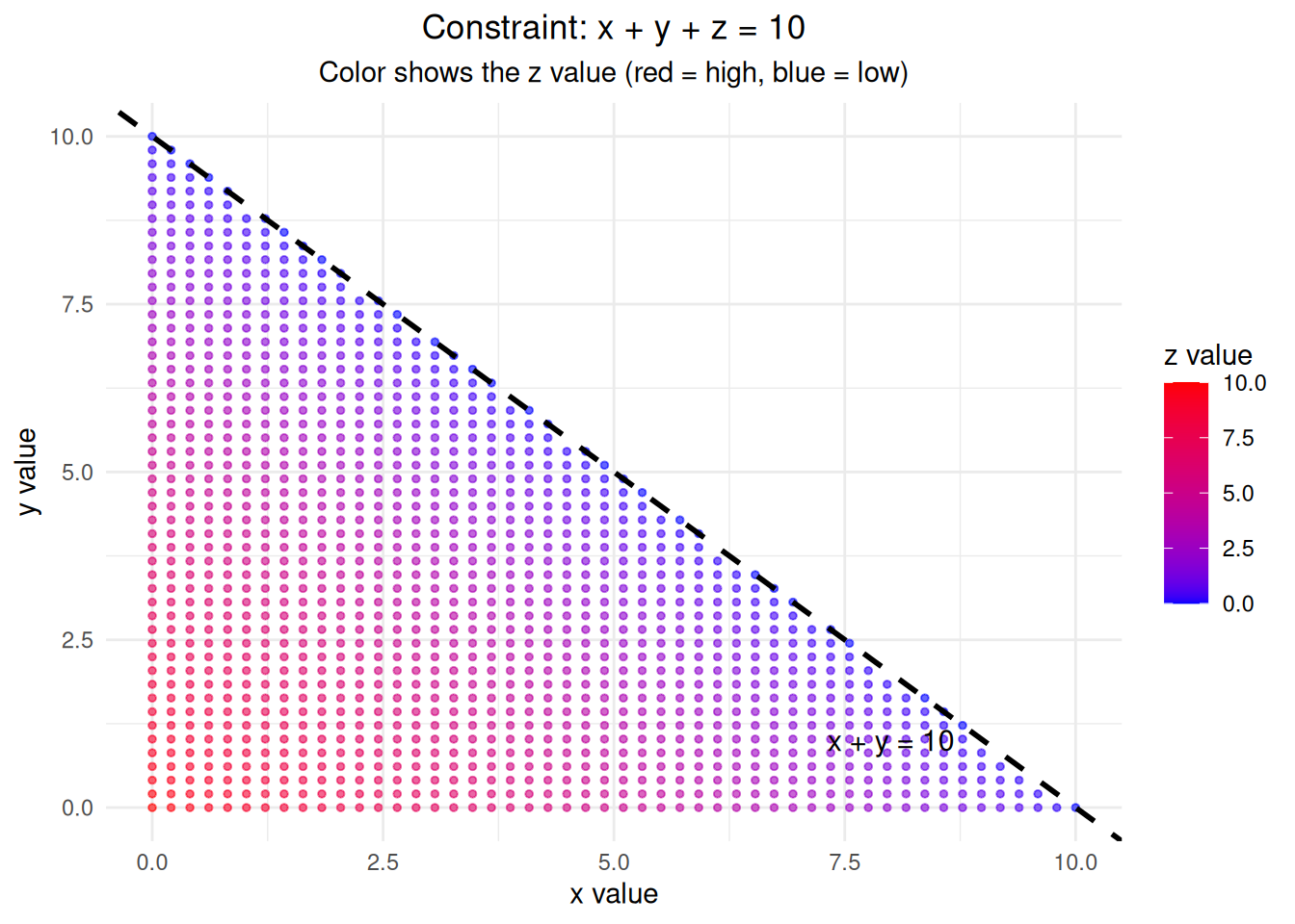

Degrees of Freedom in Sample Variance

The Key Insight: Sample Mean Constrains the Data

When we calculate sample variance, we use the sample mean as an estimate of the population mean. This creates a constraint that reduces our degrees of freedom.

# Generate sample data
sample_data <- c(2, 4, 6, 8, 10)
n <- length(sample_data)
sample_mean <- mean(sample_data)

cat("Sample data:", paste(sample_data, collapse = ", "), "\n")

Sample data: 2, 4, 6, 8, 10 

cat("Sample mean:", sample_mean, "\n")

Sample mean: 6 

cat("Sample size (n):", n, "\n")

Sample size (n): 5 

cat("Degrees of freedom for variance:", n - 1, "\n\n")

Degrees of freedom for variance: 4 

# Show why we lose 1 degree of freedom
cat("If we know the mean and n-1 values, the last value is determined:\n")

If we know the mean and n-1 values, the last value is determined:

known_values <- sample_data[1:(n-1)]
last_value <- n * sample_mean - sum(known_values)
cat("Known values:", paste(known_values, collapse = ", "), "\n")

Known values: 2, 4, 6, 8 

cat("Last value MUST be:", last_value, "\n")

Last value MUST be: 10 

cat("This is why df = n - 1 for sample variance\n")

This is why df = n - 1 for sample variance

Visualizing the Constraint in Sample Variance

# Create visualization of the constraint
df_sample <- data.frame(
  x = 1:n,
  y = sample_data,
  point_type = "Data"
)

# Add the mean line
df_mean <- data.frame(
  x = c(0.5, n + 0.5),
  y = c(sample_mean, sample_mean),
  point_type = "Mean"
)

# Combine data
df_combined <- rbind(df_sample, df_mean)

# Create plot
ggplot(df_combined, aes(x = x, y = y, color = point_type)) +
  geom_point(size = 3) +
  geom_line(data = df_mean, linewidth = 2, linetype = "dashed") +
  geom_segment(data = df_sample, aes(xend = x, yend = sample_mean), 
               color = "red", alpha = 0.5) +
  labs(title = "Sample Data with Mean Constraint",
       subtitle = "Red lines show deviations from mean",
       x = "Observation", y = "Value",
       color = "Type") +
  theme_minimal() +
  theme(plot.title = element_text(hjust = 0.5),
        plot.subtitle = element_text(hjust = 0.5)) +
  scale_color_manual(values = c("Data" = "blue", "Mean" = "red"))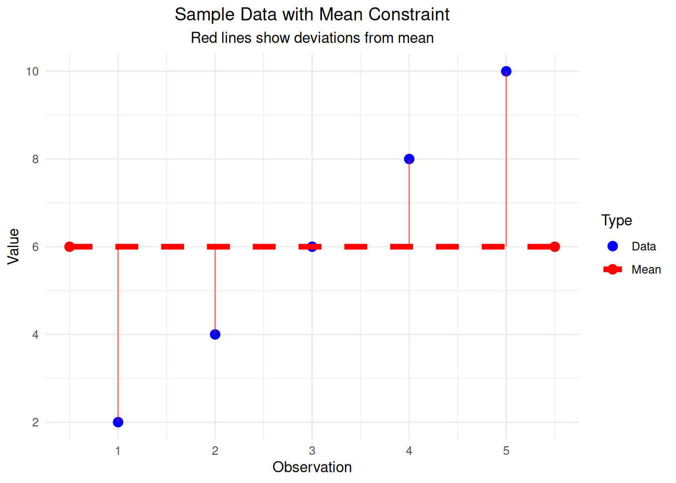

Degrees of Freedom in Different Contexts

1. One-Sample t-test

# Simulate one-sample t-test
population_mean <- 100
sample_size <- 15
sample_data <- rnorm(sample_size, mean = 105, sd = 10)

# Calculate t-statistic
sample_mean <- mean(sample_data)
sample_se <- sd(sample_data) / sqrt(sample_size)
t_stat <- (sample_mean - population_mean) / sample_se
df_t <- sample_size - 1

cat("One-Sample t-test:\n")

One-Sample t-test:

cat("Sample size:", sample_size, "\n")

Sample size: 15 

cat("Degrees of freedom:", df_t, "\n")

Degrees of freedom: 14 

cat("t-statistic:", round(t_stat, 3), "\n")

t-statistic: 2.989 

cat("p-value:", round(2 * pt(-abs(t_stat), df_t), 4), "\n")

p-value: 0.0098 

2. Two-Sample t-test

# Simulate two-sample t-test
n1 <- 12
n2 <- 10
group1 <- rnorm(n1, mean = 100, sd = 8)
group2 <- rnorm(n2, mean = 105, sd = 8)

# Calculate pooled t-test
mean1 <- mean(group1)
mean2 <- mean(group2)
var1 <- var(group1)
var2 <- var(group2)

# Pooled variance
pooled_var <- ((n1 - 1) * var1 + (n2 - 1) * var2) / (n1 + n2 - 2)
pooled_se <- sqrt(pooled_var * (1/n1 + 1/n2))
t_stat_pooled <- (mean1 - mean2) / pooled_se
df_pooled <- n1 + n2 - 2

cat("Two-Sample t-test (pooled):\n")

Two-Sample t-test (pooled):

cat("Group 1 size:", n1, "\n")

Group 1 size: 12 

cat("Group 2 size:", n2, "\n")

Group 2 size: 10 

cat("Degrees of freedom:", df_pooled, "\n")

Degrees of freedom: 20 

cat("t-statistic:", round(t_stat_pooled, 3), "\n")

t-statistic: -3.414 

cat("p-value:", round(2 * pt(-abs(t_stat_pooled), df_pooled), 4), "\n")

p-value: 0.0028 

Visualizing t-Distributions with Different Degrees of Freedom

# Create t-distributions with different degrees of freedom
x_vals <- seq(-4, 4, length.out = 200)
df_values <- c(1, 3, 10, 30)

# Calculate t-distribution densities
t_densities <- data.frame()
for(df in df_values) {
  density_vals <- dt(x_vals, df = df)
  t_densities <- rbind(t_densities, 
                       data.frame(x = x_vals, density = density_vals, df = paste("df =", df)))
}

# Add normal distribution for comparison
normal_density <- dnorm(x_vals, mean = 0, sd = 1)
t_densities <- rbind(t_densities, 
                     data.frame(x = x_vals, density = normal_density, df = "Normal"))

# Create plot
ggplot(t_densities, aes(x = x, y = density, color = df)) +
  geom_line(linewidth = 1) +
  labs(title = "t-Distributions with Different Degrees of Freedom",
       subtitle = "As df increases, t-distribution approaches normal",
       x = "Value", y = "Density",
       color = "Distribution") +
  theme_minimal() +
  theme(plot.title = element_text(hjust = 0.5),
        plot.subtitle = element_text(hjust = 0.5)) +
  scale_color_brewer(palette = "Set1")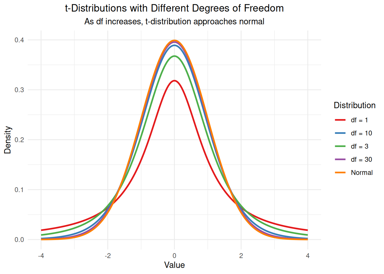

Degrees of Freedom in Chi-Square Tests

Chi-Square Goodness of Fit

# Simulate chi-square goodness of fit test
observed <- c(22, 18, 25, 15, 20)  # Observed counts
expected <- rep(20, 5)  # Expected counts (equal probability)

# Calculate chi-square statistic
chi_sq <- sum((observed - expected)^2 / expected)
df_chi <- length(observed) - 1  # k - 1 categories

cat("Chi-Square Goodness of Fit Test:\n")

Chi-Square Goodness of Fit Test:

cat("Number of categories:", length(observed), "\n")

Number of categories: 5 

cat("Degrees of freedom:", df_chi, "\n")

Degrees of freedom: 4 

cat("Chi-square statistic:", round(chi_sq, 3), "\n")

Chi-square statistic: 2.9 

cat("p-value:", round(1 - pchisq(chi_sq, df_chi), 4), "\n")

p-value: 0.5747 

Visualizing Chi-Square Distributions

# Create chi-square distributions with different degrees of freedom
x_vals <- seq(0, 20, length.out = 200)
df_values_chi <- c(1, 2, 5, 10)

# Calculate chi-square distribution densities
chi_densities <- data.frame()
for(df in df_values_chi) {
  density_vals <- dchisq(x_vals, df = df)
  chi_densities <- rbind(chi_densities, 
                         data.frame(x = x_vals, density = density_vals, df = paste("df =", df)))
}

# Create plot
ggplot(chi_densities, aes(x = x, y = density, color = df)) +
  geom_line(linewidth = 1) +
  labs(title = "Chi-Square Distributions with Different Degrees of Freedom",
       subtitle = "Shape becomes more symmetric as df increases",
       x = "Value", y = "Density",
       color = "Degrees of Freedom") +
  theme_minimal() +
  theme(plot.title = element_text(hjust = 0.5),
        plot.subtitle = element_text(hjust = 0.5)) +
  scale_color_brewer(palette = "Set1")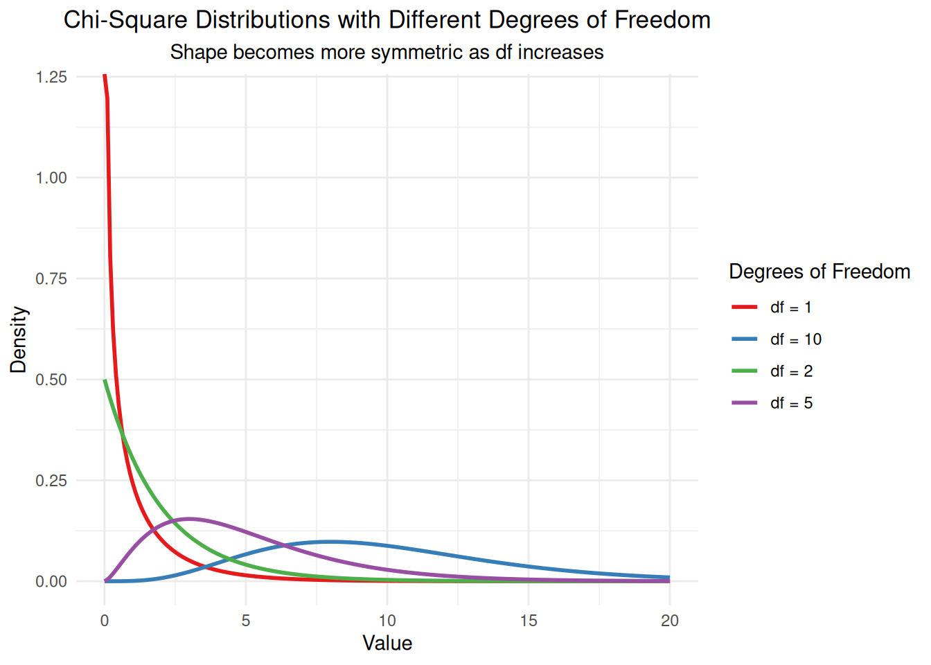

Degrees of Freedom in Regression

Simple Linear Regression

# Generate data for simple linear regression
n_reg <- 20
x_reg <- seq(1, 10, length.out = n_reg)
y_reg <- 2 + 1.5 * x_reg + rnorm(n_reg, 0, 2)

# Fit regression model
lm_model <- lm(y_reg ~ x_reg)
residuals <- residuals(lm_model)

# Degrees of freedom
df_total <- n_reg - 1      # Total df
df_model <- 1              # Model df (one slope parameter)
df_residual <- n_reg - 2   # Residual df

cat("Simple Linear Regression:\n")

Simple Linear Regression:

cat("Sample size:", n_reg, "\n")

Sample size: 20 

cat("Total df:", df_total, "\n")

Total df: 19 

cat("Model df:", df_model, "\n")

Model df: 1 

cat("Residual df:", df_residual, "\n")

Residual df: 18 

cat("R-squared:", round(summary(lm_model)$r.squared, 3), "\n")

R-squared: 0.848 

Visualizing Regression Degrees of Freedom

# Create regression plot
df_reg <- data.frame(x = x_reg, y = y_reg)

ggplot(df_reg, aes(x = x, y = y)) +
  geom_point(size = 3, color = "blue") +
  geom_smooth(method = "lm", color = "red", linewidth = 1) +
  geom_segment(aes(xend = x, yend = fitted(lm_model)), 
               color = "green", alpha = 0.5) +
  labs(title = "Simple Linear Regression",
       subtitle = "Green lines show residuals (constrained by regression line)",
       x = "X", y = "Y") +
  theme_minimal() +
  theme(plot.title = element_text(hjust = 0.5),
        plot.subtitle = element_text(hjust = 0.5))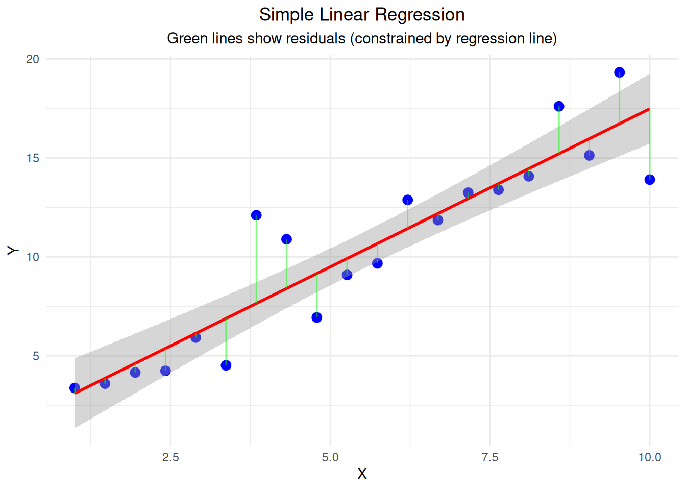

Interactive Example: Degrees of Freedom Calculator

# Function to demonstrate degrees of freedom
demonstrate_df <- function(n, constraint_type = "mean") {
  
  if(constraint_type == "mean") {
    # Generate n random numbers
    data <- rnorm(n, mean = 10, sd = 2)
    
    # Show how the last value is constrained
    if(n > 1) {
      known_values <- data[1:(n-1)]
      target_mean <- mean(data)
      last_value <- n * target_mean - sum(known_values)
      
      cat("Degrees of Freedom Demonstration:\n")
      cat("Sample size:", n, "\n")
      cat("Constraint: Sample mean =", round(target_mean, 2), "\n")
      cat("Known values:", paste(round(known_values, 2), collapse = ", "), "\n")
      cat("Last value MUST be:", round(last_value, 2), "\n")
      cat("Degrees of freedom =", n - 1, "\n")
    }
  }
}

# Demonstrate with different sample sizes
demonstrate_df(5, "mean")

Degrees of Freedom Demonstration:
Sample size: 5 
Constraint: Sample mean = 10.32 
Known values: 11.17, 10.25, 10.43, 10.76 
Last value MUST be: 9 
Degrees of freedom = 4 

cat("\n")

demonstrate_df(10, "mean")

Degrees of Freedom Demonstration:
Sample size: 10 
Constraint: Sample mean = 9.71 
Known values: 9.33, 7.96, 7.86, 10.61, 10.9, 10.11, 11.84, 14.1, 9.02 
Last value MUST be: 5.38 
Degrees of freedom = 9 

Key Takeaways

Why Degrees of Freedom Matter:

1. Corrects for bias: Using n-1 instead of n in sample variance gives an unbiased estimate
2. Accounts for constraints: Each constraint reduces the number of independent pieces of information
3. Affects statistical tests: Different degrees of freedom lead to different critical values
4. Determines distribution shape: Higher degrees of freedom make distributions more normal

Common Rules:

• Sample variance: df = n - 1
• One-sample t-test: df = n - 1
• Two-sample t-test: df = n₁ + n₂ - 2
• Chi-square goodness of fit: df = k - 1 (k categories)
• Simple linear regression: df_residual = n - 2

The Intuition:

Think of degrees of freedom as the number of “free choices” you have after accounting for the constraints imposed by your statistical procedure. Each constraint reduces your degrees of freedom by one.