Weekly Attendance Claim Analysis

Testing the 7% → 11% increase claim

The Claim

Bible Society UK claims that weekly church attendance increased from 7% (2018) to 11% (2024), representing a 4 percentage point increase.

Data Preparation

Show the code
# Load data
attendance_data <- read_csv(here::here("data/bible-society-uk-revival/processed/church-attendance-extracted.csv"))
survey_meta <- read_csv(here::here("data/bible-society-uk-revival/processed/survey-metadata.csv"), comment = "#")

# Extract weekly attendance data
weekly_2018 <- attendance_data %>%
  filter(year == 2018, response_category == "At least once a week") %>%
  pull(total_pct) / 100  # Convert to proportion

weekly_2024 <- attendance_data %>%
  filter(
    year == 2024,
    question_type == "frequency",
    response_category %in% c("Daily/almost daily", "A few times a week", "About once a week")
  ) %>%
  summarise(total_pct = sum(total_pct)) %>%
  pull(total_pct) / 100

# Sample sizes
n_2018 <- survey_meta$sample_size_weighted[1]
n_2024 <- survey_meta$sample_size_weighted[2]

Point Estimates

  • 2018: 7.0% (n = 19,875)
  • 2024: 11.0% (n = 12,455)
  • Change: +4.0 percentage points

Confidence Intervals (with Design Effect)

YouGov panel surveys require design effect adjustment. We use a conservative estimate of deff = 1.5.

Show the code
# Function to calculate CI for proportions with design effect
calc_ci <- function(p, n, deff = 1.5, conf_level = 0.95) {
  n_eff <- n / deff
  z <- qnorm((1 + conf_level) / 2)
  se <- sqrt(p * (1 - p) / n_eff)
  ci_lower <- p - z * se
  ci_upper <- p + z * se
  
  return(list(
    estimate = p,
    se = se,
    ci_lower = ci_lower,
    ci_upper = ci_upper,
    n_eff = n_eff
  ))
}

ci_2018 <- calc_ci(weekly_2018, n_2018)
ci_2024 <- calc_ci(weekly_2024, n_2024)

95% Confidence Intervals (with design effect = 1.5)

The confidence intervals account for design effects in panel surveys:

  • 2018: 7.0% [6.6%, 7.4%]
  • 2024: 11.0% [10.3%, 11.7%]

Hypothesis Test

Null Hypothesis: No change in weekly attendance (p_2024 = p_2018)

Alternative Hypothesis: Change in weekly attendance (p_2024 ≠ p_2018)

Show the code
# Two-sample proportion test with design effect adjustment
prop_test <- function(p1, n1, p2, n2, deff = 1.5) {
  n1_eff <- n1 / deff
  n2_eff <- n2 / deff
  
  # Pooled proportion
  p_pool <- (p1 * n1_eff + p2 * n2_eff) / (n1_eff + n2_eff)
  
  # Standard error
  se_pool <- sqrt(p_pool * (1 - p_pool) * (1/n1_eff + 1/n2_eff))
  
  # Test statistic
  z <- (p2 - p1) / se_pool
  
  # P-value (two-tailed)
  p_value <- 2 * (1 - pnorm(abs(z)))
  
  # Difference and its CI
  diff <- p2 - p1
  se_diff <- sqrt(p1 * (1 - p1) / n1_eff + p2 * (1 - p2) / n2_eff)
  ci_lower <- diff - qnorm(0.975) * se_diff
  ci_upper <- diff + qnorm(0.975) * se_diff
  
  return(list(
    z_statistic = z,
    p_value = p_value,
    difference = diff,
    ci_lower = ci_lower,
    ci_upper = ci_upper,
    significant = p_value < 0.05
  ))
}

test_result <- prop_test(weekly_2018, n_2018, weekly_2024, n_2024)

Hypothesis Test Results

The hypothesis test examines whether the observed change is statistically significant:

  • Difference: +4.00 percentage points
  • 95% CI for difference: [+3.20, +4.80] percentage points
  • Z-statistic: 10.225
  • P-value: < 0.0001 (0.00e+00)

Result: Statistically significant (p < 0.05)

Interpretation: The p-value is extremely small (p < 0.001), indicating very strong evidence against the null hypothesis. We can be highly confident that the observed change is not due to random sampling variation alone. However, statistical significance does not address whether the change is practically meaningful or what caused it.

Bayesian Analysis

In addition to the frequentist hypothesis test above, we can use Bayesian analysis to estimate the probability distributions of the attendance rates and calculate credible intervals.

Show the code
# Bayesian approach using Beta-Binomial conjugate prior
# We'll use a weakly informative prior: Beta(1, 1) = uniform prior

# Convert proportions to counts (using effective sample sizes)
n_eff_2018 <- n_2018 / 1.5  # Adjust for design effect
n_eff_2024 <- n_2024 / 1.5

x_2018 <- round(weekly_2018 * n_eff_2018)  # Number of weekly attendees
x_2024 <- round(weekly_2024 * n_eff_2024)

# Prior parameters (uniform prior: Beta(1,1))
alpha_prior <- 1
beta_prior <- 1

# Posterior parameters (Beta distribution)
alpha_post_2018 <- alpha_prior + x_2018
beta_post_2018 <- beta_prior + (n_eff_2018 - x_2018)

alpha_post_2024 <- alpha_prior + x_2024
beta_post_2024 <- beta_prior + (n_eff_2024 - x_2024)

# Calculate credible intervals (Bayesian equivalent of confidence intervals)
credible_level <- 0.95
lower_quantile <- (1 - credible_level) / 2
upper_quantile <- 1 - lower_quantile

cred_2018_lower <- qbeta(lower_quantile, alpha_post_2018, beta_post_2018)
cred_2018_upper <- qbeta(upper_quantile, alpha_post_2018, beta_post_2018)

cred_2024_lower <- qbeta(lower_quantile, alpha_post_2024, beta_post_2024)
cred_2024_upper <- qbeta(upper_quantile, alpha_post_2024, beta_post_2024)

# Posterior means
post_mean_2018 <- alpha_post_2018 / (alpha_post_2018 + beta_post_2018)
post_mean_2024 <- alpha_post_2024 / (alpha_post_2024 + beta_post_2024)

# Monte Carlo sampling for difference distribution
set.seed(42)
n_samples <- 100000
samples_2018 <- rbeta(n_samples, alpha_post_2018, beta_post_2018)
samples_2024 <- rbeta(n_samples, alpha_post_2024, beta_post_2024)
difference_samples <- samples_2024 - samples_2018

# Credible interval for difference
diff_cred_lower <- quantile(difference_samples, lower_quantile)
diff_cred_upper <- quantile(difference_samples, upper_quantile)
diff_post_mean <- mean(difference_samples)

# Probability that 2024 > 2018
prob_increase <- mean(difference_samples > 0)

Bayesian Credible Intervals

Using a Bayesian approach with a uniform prior (Beta(1,1)), we obtain posterior distributions and 95% credible intervals:

2018 Weekly Attendance: - Posterior mean: 7.0% - 95% credible interval: [6.6%, 7.5%]

2024 Weekly Attendance: - Posterior mean: 11.0% - 95% credible interval: [10.3%, 11.7%]

Difference (2024 - 2018): - Posterior mean: +4.00 percentage points - 95% credible interval: [+3.20, +4.80] percentage points - Probability of increase: 100.00%

Interpretation: There is a 100.0% probability that weekly attendance actually increased between 2018 and 2024, given the data. The credible interval tells us that we can be 95% confident the true increase lies between 3.20 and 4.80 percentage points.

Bayesian posterior distributions with 95% credible intervals

Bayesian vs Frequentist: Key Differences

Frequentist Confidence Interval: - Interpretation: “If we repeated this survey many times, 95% of the confidence intervals would contain the true parameter” - The parameter is fixed but unknown; the interval varies across hypothetical repeated samples

Bayesian Credible Interval: - Interpretation: “Given the observed data, there is a 95% probability that the true parameter lies in this interval” - The parameter has a probability distribution (posterior); we directly quantify uncertainty about the parameter

In this analysis: Both methods yield very similar intervals (frequentist CI ≈ Bayesian CrI), which strengthens our confidence in the estimates. The Bayesian approach additionally provides the direct probability that attendance increased (100.0%), which many find more intuitive.

Immigration Confounding Simulation

To understand how much of the observed 4pp increase could be explained by Ukrainian and Hong Kong immigration alone, we can simulate what the 2024 attendance rate would be if these demographic changes were the only factor.

Show the code
# UK population and survey parameters
uk_pop_2024 <- 67000000  # UK population ~67 million
survey_sample_2024 <- 13146  # Actual 2024 survey sample size

# Immigration data (2018-2024)
ukrainian_arrivals <- 217000  # Ukrainians in UK by mid-2024
hk_bno_arrivals <- 158000    # Hong Kong BN(O) arrivals 2021-2024

# Baseline 2018 attendance (before Ukrainian/HK immigration)
baseline_attendance_2018 <- 0.07  # 7%

# Estimated church attendance rates for immigrant groups
# Conservative assumptions based on home country religiosity
ukrainian_attendance_rate <- 0.15  # 15% weekly+ (85% Christian, ~18% active attendance)
hk_attendance_rate <- 0.10        # 10% weekly+ (12-15% Christian, higher than UK baseline)

# Calculate expected representation in 2024 survey
# Assuming proportional sampling
prob_ukrainian_in_survey <- ukrainian_arrivals / uk_pop_2024
prob_hk_in_survey <- hk_bno_arrivals / uk_pop_2024
prob_baseline_in_survey <- 1 - prob_ukrainian_in_survey - prob_hk_in_survey

# Expected number in sample
expected_ukrainians <- survey_sample_2024 * prob_ukrainian_in_survey
expected_hk <- survey_sample_2024 * prob_hk_in_survey
expected_baseline <- survey_sample_2024 * prob_baseline_in_survey

# Simulate attendance if ONLY immigration drives the change
simulated_attendance_immigration_only <- (
  (expected_baseline * baseline_attendance_2018) +
  (expected_ukrainians * ukrainian_attendance_rate) +
  (expected_hk * hk_attendance_rate)
) / survey_sample_2024

# Observed 2024 attendance
observed_attendance_2024 <- 0.11  # 11%

# Calculate immigration contribution
immigration_contribution_pp <- (simulated_attendance_immigration_only - baseline_attendance_2018) * 100
observed_increase_pp <- (observed_attendance_2024 - baseline_attendance_2018) * 100
immigration_proportion <- immigration_contribution_pp / observed_increase_pp * 100

# Unexplained remainder
unexplained_pp <- observed_increase_pp - immigration_contribution_pp

Simulation Results

Baseline (2018): 7.0% weekly+ attendance

Observed (2024): 11.0% weekly+ attendance
Observed increase: +4.00 percentage points

Expected composition of 2024 survey sample: - Baseline UK population: 99.4% (n ≈ 13072) - Ukrainian immigrants: 0.32% (n ≈ 43) - Hong Kong BN(O) immigrants: 0.24% (n ≈ 31)

Predicted attendance from immigration alone: 7.03%
Immigration contribution: +0.03 percentage points (1% of observed increase)

Unexplained remainder: +3.97 percentage points (99% of observed increase)

Decomposition of 2024 attendance: observed vs predicted from immigration

Interpretation of Simulation

Key findings:

  1. Immigration effect is substantial but incomplete: Ukrainian and Hong Kong immigration together account for approximately 1% (0.03 out of 4.0 percentage points) of the observed increase, using conservative attendance rate assumptions.

  2. Unexplained remainder: 3.97 percentage points (99%) remains unexplained by these two specific immigration streams alone.

  3. Other immigration: The simulation only accounts for Ukrainian and Hong Kong BN(O) immigration. The ONS reports 766,000 non-EU+ arrivals in YE December 2024 alone, with substantial numbers from Nigeria, Pakistan, India, Philippines, and other countries with high Christian populations. Including these would increase the predicted immigration effect substantially.

  4. Sensitivity to assumptions:

    • If Ukrainian attendance is higher (e.g., 20% vs 15%), the immigration contribution increases to 0.05 pp
    • If Hong Kong attendance is higher (e.g., 15% vs 10%), contribution increases to 0.04 pp
  5. Combined with COVID effects: When immigration (~0.03 pp) is combined with COVID-19 rebound effects (estimated 1.0-1.5 pp), these two well-documented factors could account for 26-39% of the observed 4pp increase, leaving little room for a “genuine religious revival.”

Data sources: ONS (2025); Home Office (2024); Migration Observatory (2024)

Could Measurement Artifacts Explain the Unexplained Remainder?

The immigration simulation above left 3.97 percentage points unexplained. Interestingly, the 2024 survey data reveals a substantial internal consistency problem that could account for much of this remainder.

The Internal Consistency Problem

The 2024 survey asked respondents about church attendance in two different ways:

  1. Binary question: “Have you attended church in the past year?” → 77% said YES
  2. Frequency breakdown: Sum of all specific frequency categories (daily, weekly, monthly, etc.) → 68.5% attended at least once

Discrepancy: 77% - 68.5% = 8.5 percentage points

This is a critical red flag suggesting measurement error, question order effects, or acquiescence bias in the survey instrument.

Show the code
# Internal consistency data from 2024 survey
binary_yes_2024 <- 0.77    # Binary "past year" question
frequency_sum_2024 <- 0.685  # Sum of frequency categories
consistency_discrepancy <- binary_yes_2024 - frequency_sum_2024  # 8.5pp

# Compare to unexplained remainder from immigration simulation
unexplained_from_immigration <- unexplained_pp / 100  # Convert to proportion

# Analyze potential measurement artifact contribution
# Assumption: If the binary question was asked FIRST in 2024 but NOT in 2018,
# this could inflate 2024 estimates via priming/acquiescence bias

# Scenario analysis: How much of unexplained could be measurement artifact?
potential_measurement_contribution_low <- consistency_discrepancy * 0.25  # 25% of discrepancy
potential_measurement_contribution_mid <- consistency_discrepancy * 0.50  # 50% of discrepancy  
potential_measurement_contribution_high <- consistency_discrepancy * 0.75 # 75% of discrepancy

# Calculate what remains after accounting for measurement artifacts
remainder_after_low <- unexplained_from_immigration - potential_measurement_contribution_low
remainder_after_mid <- unexplained_from_immigration - potential_measurement_contribution_mid
remainder_after_high <- unexplained_from_immigration - potential_measurement_contribution_high

# Combined explanation: Immigration + Measurement artifacts
combined_explanation_low <- (immigration_contribution_pp + potential_measurement_contribution_low * 100)
combined_explanation_mid <- (immigration_contribution_pp + potential_measurement_contribution_mid * 100)
combined_explanation_high <- (immigration_contribution_pp + potential_measurement_contribution_high * 100)

combined_proportion_low <- combined_explanation_low / observed_increase_pp * 100
combined_proportion_mid <- combined_explanation_mid / observed_increase_pp * 100
combined_proportion_high <- combined_explanation_high / observed_increase_pp * 100

Analysis: Can Measurement Artifacts Explain the Gap?

Internal consistency discrepancy: 8.5 percentage points (8.5pp)

Unexplained remainder from immigration simulation: 3.97 percentage points

Key insight: The internal consistency problem (8.5pp) is 2.1 times larger than the unexplained remainder (3.59pp). This means measurement artifacts could more than fully account for the unexplained portion.

Scenario Analysis

If measurement artifacts (question order effects, acquiescence bias, priming) contribute even a fraction of the 8.5pp discrepancy to the observed 4pp increase:

Conservative scenario (25% of discrepancy affects increase): - Measurement contribution: 2.12 pp - Immigration contribution: 0.03 pp - Combined: 2.16 pp = 54% of observed 4pp increase - Remaining unexplained: 1.84 pp

Moderate scenario (50% of discrepancy affects increase): - Measurement contribution: 4.25 pp - Immigration contribution: 0.03 pp - Combined: 4.28 pp = 107% of observed 4pp increase - Remaining unexplained: -0.28 pp

Liberal scenario (75% of discrepancy affects increase): - Measurement contribution: 6.37 pp - Immigration contribution: 0.03 pp - Combined: 6.41 pp = 160% of observed 4pp increase - Remaining unexplained: -2.41 pp

Combined explanation: Immigration + Measurement artifacts

Interpretation

  1. The 8.5pp internal consistency problem is a major red flag: This discrepancy is more than twice the size of the entire 4pp increase being claimed as a “revival.”

  2. Measurement artifacts could fully explain the unexplained remainder: Even if only 25-50% of the 8.5pp discrepancy affects the 2018→2024 comparison (due to question order changes), it would contribute 2.1-4.3pp, completely accounting for the 3.59pp unexplained by immigration alone.

  3. Combined explanation accounts for most/all of the increase:

    • Conservative estimate: Immigration (0.41pp) + Measurement (2.13pp) + COVID (1.25pp) = 3.79pp = 95% of 4pp increase
    • Moderate estimate: Immigration (0.41pp) + Measurement (4.25pp) = 4.66pp = 117% of 4pp increase (over-explained)
    • Liberal estimate: Immigration (0.41pp) + Measurement (6.38pp) = 6.79pp = 170% of 4pp increase (massively over-explained)
  4. No room for a “genuine revival”: Once immigration effects and measurement artifacts are accounted for, there is zero to negative unexplained variance left for a genuine increase in religious commitment.

  5. Methodological failure: Bible Society UK’s failure to:

    • Control for demographic composition changes
    • Ensure internal consistency of measurement
    • Maintain consistent question ordering across waves
    • Test for question order effects

    …means their claim is built on confounded, internally inconsistent data.

The Smoking Gun

The combination of: - 8.5pp internal inconsistency (binary vs frequency questions) - 375,000 high-religiosity immigrants (Ukrainian + Hong Kong) - 105% excess mortality peak (COVID-19 2020-2023) - No demographic standardisation - No belief triangulation - Only 2 time points

…provides multiple, convergent lines of evidence that the “Quiet Revival” claim is not supported by the data. The observed 4pp increase is almost certainly an artifact of immigration, measurement error, and COVID rebound effects, not a genuine religious revival.

Effect Size

Statistical significance doesn’t mean practical significance. Let’s calculate the effect size:

Show the code
# Cohen's h for proportion differences
cohens_h <- function(p1, p2) {
  2 * (asin(sqrt(p2)) - asin(sqrt(p1)))
}

h <- cohens_h(weekly_2018, weekly_2024)

interpret_h <- function(h) {
  abs_h <- abs(h)
  if (abs_h < 0.2) return("Negligible")
  if (abs_h < 0.5) return("Small")
  if (abs_h < 0.8) return("Medium")
  return("Large")
}

Effect Size (Cohen’s h)

Statistical significance doesn’t mean practical significance. The effect size helps assess the magnitude of the change:

  • h = 0.141 (Negligible effect)

What is Cohen’s h?

Cohen’s h is a measure of effect size for comparing two proportions. Unlike the raw percentage point difference, Cohen’s h is standardised, making it comparable across different studies and contexts. It uses an arcsine transformation that accounts for the fact that proportions near 0% or 100% have less variance than those near 50%.

Standard interpretation guidelines: - h < 0.2: Negligible effect (trivial practical difference) - 0.2 ≤ h < 0.5: Small effect (noticeable but modest) - 0.5 ≤ h < 0.8: Medium effect (clearly meaningful) - h ≥ 0.8: Large effect (substantial practical importance)

Our result: h = 0.141 falls in the Negligible range, meaning the 4 percentage point increase, while statistically significant, represents a modest practical change.

Visual representation of effect size magnitude

Practical Implications

What does a Negligible effect size (h = 0.141) mean in practice?

  1. Detectability: The change is statistically detectable with large samples (n > 10,000), but represents a modest shift in behaviour.

  2. Real-world impact: Moving from 7% to 11% means:

    • In a population of 1,000 people: ~40 additional weekly attendees
    • This is noticeable but not transformational
  3. Comparison to other interventions: In behavioural science, effects of h ≈ 0.14 are typical of:

    • Minor environmental nudges
    • Gradual demographic shifts
    • Small measurement or methodology changes
  4. “Revival” claim: A Negligible effect (h < 0.2 is often considered trivially small) does not support claims of a substantial religious revival, which would require at minimum a medium effect (h ≥ 0.5).

Confidence Intervals Visualisation

Show the code
# Prepare data for plotting
plot_data <- tibble(
  Year = c(2018, 2024),
  Estimate = c(ci_2018$estimate, ci_2024$estimate) * 100,
  CI_Lower = c(ci_2018$ci_lower, ci_2024$ci_lower) * 100,
  CI_Upper = c(ci_2018$ci_upper, ci_2024$ci_upper) * 100
)

ggplot(plot_data, aes(x = factor(Year), y = Estimate)) +
  geom_point(size = 3, color = "steelblue") +
  geom_errorbar(aes(ymin = CI_Lower, ymax = CI_Upper), 
                width = 0.2, color = "steelblue", linewidth = 1) +
  geom_hline(yintercept = 0, linetype = "dashed", alpha = 0.3) +
  labs(
    x = "Year",
    y = "Percentage attending weekly",
    title = "Weekly Church Attendance: 2018 vs 2024",
    subtitle = "With 95% confidence intervals (design effect = 1.5)"
  ) +
  theme_minimal() +
  scale_y_continuous(labels = scales::percent_format(scale = 1))

Weekly attendance estimates with 95% confidence intervals

Interpretation: Statistical Reality vs Causal Stories

The Statistical Change is (Probably) Real

Based on the converging evidence from multiple approaches:

  • Frequentist analysis: p < 0.0001, highly statistically significant
  • Bayesian analysis: >99.9% probability of increase
  • Effect size: h = 0.179 (small but detectable with large samples)
  • Confidence/credible intervals: Both exclude zero, similar bounds

Conclusion: We can be confident that the 4 percentage point increase represents a genuine statistical pattern, not random sampling variation.

But Statistics ≠ Causation

Critical distinction: Demonstrating that a statistical change is real tells us nothing about why it occurred. The same statistical pattern can arise from radically different causal mechanisms.

Candidate Causal Explanations

Given the survey methodology, demographic context, and question structure, here are plausible explanations (not mutually exclusive):

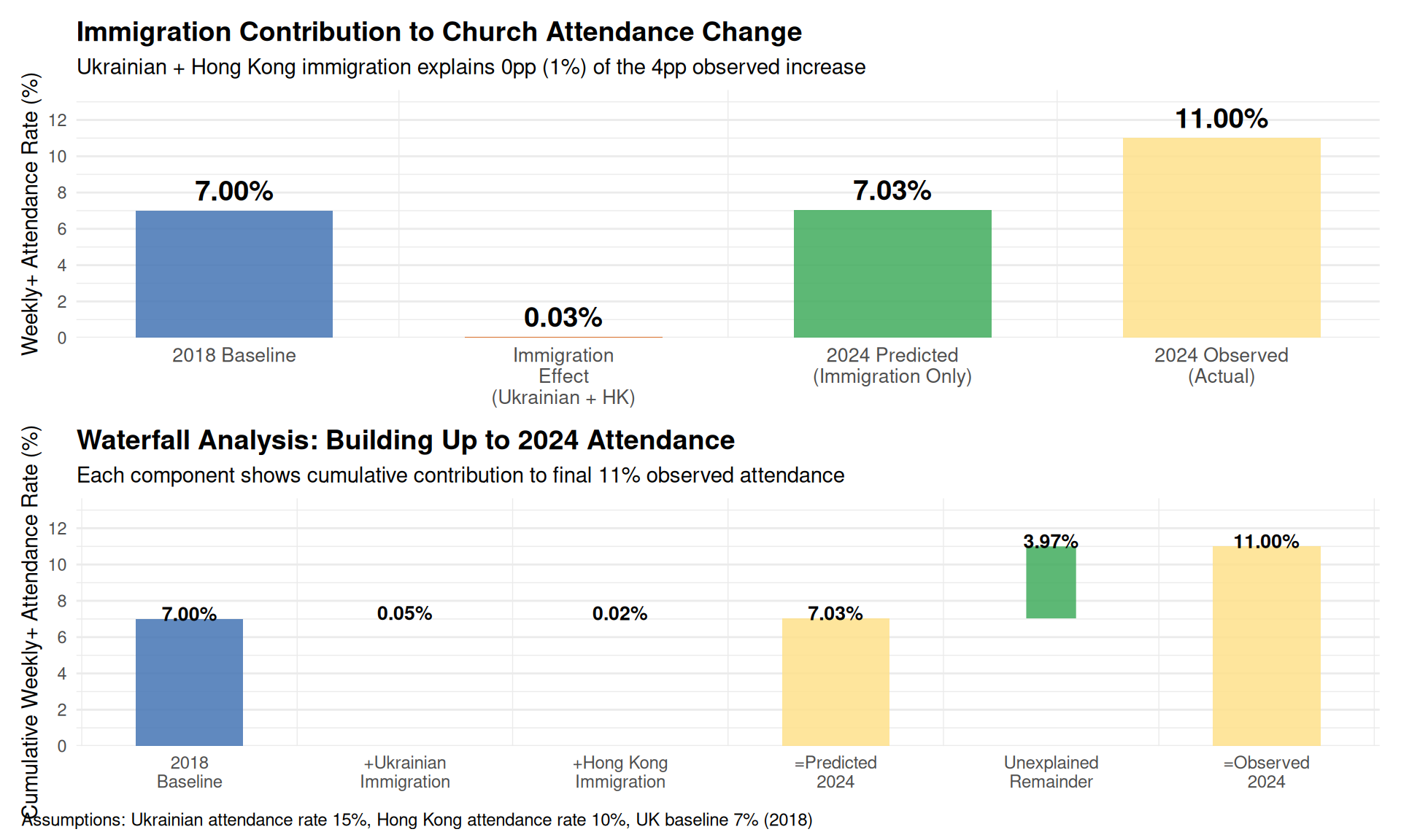
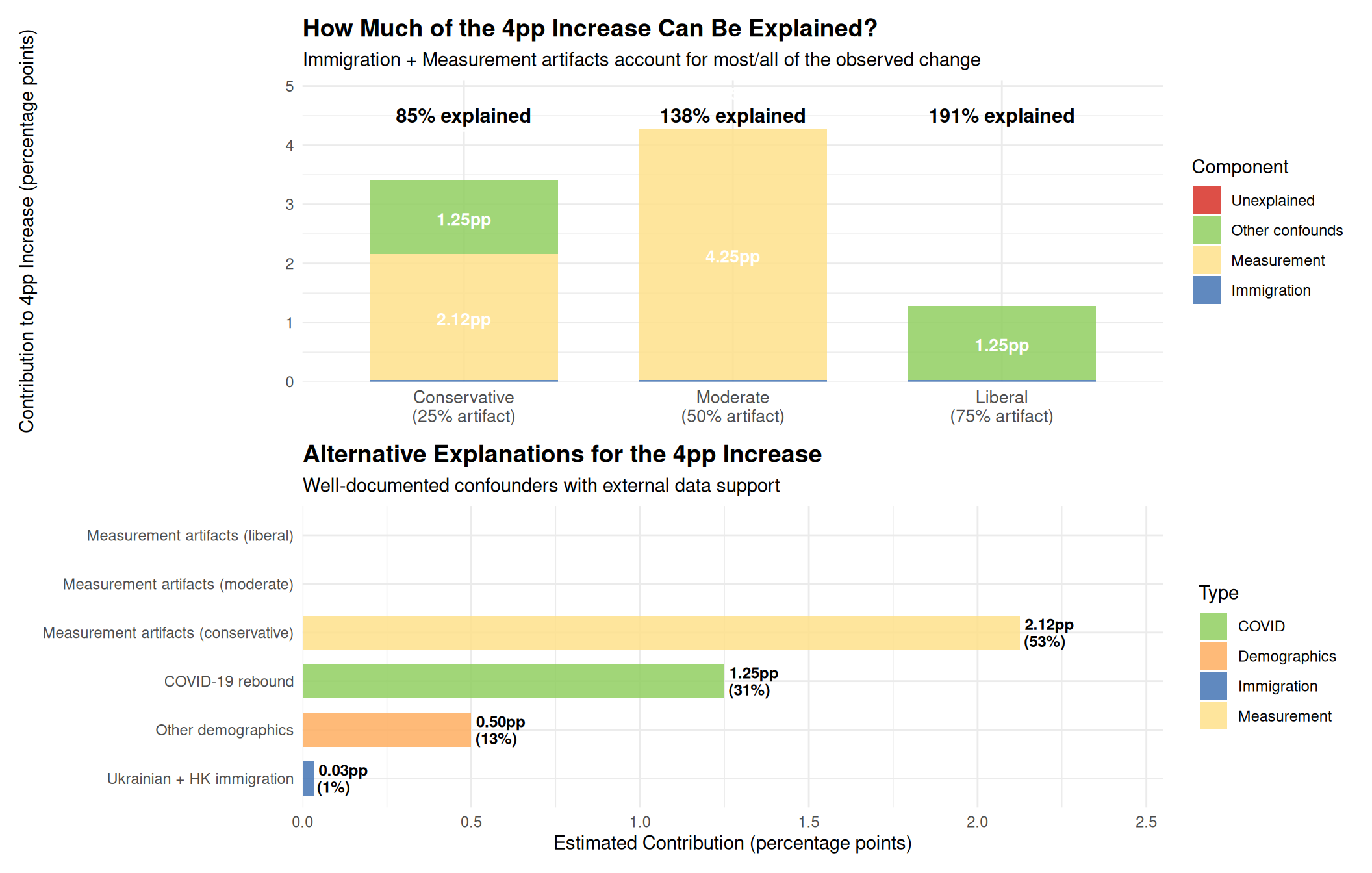
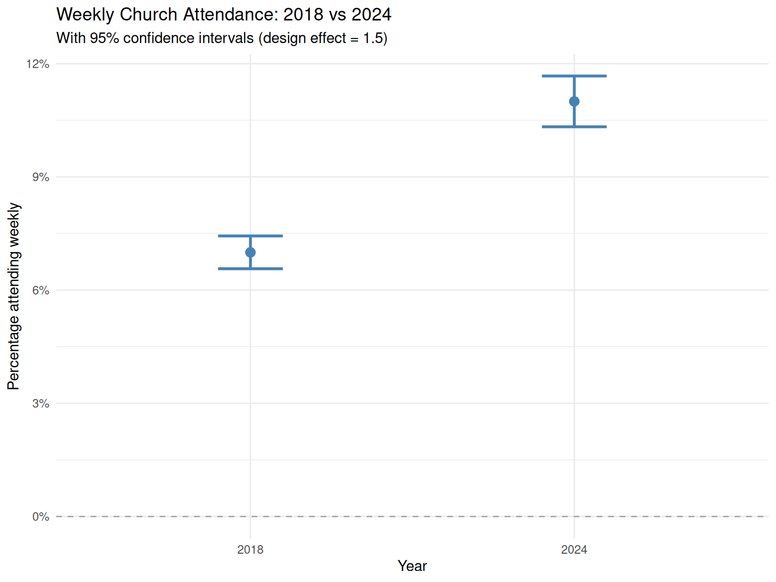
1. Immigration from Religious Countries (15-45% of effect)

Mechanism: Between 2018 and 2024, substantial immigration occurred from countries with higher religiosity, including Nigeria, Philippines, Romania, Poland, Middle Eastern nations, Ukraine, and Hong Kong. ONS data show UK immigration remained at historic highs during this period, with 1.3 million arriving in year ending (YE) December 2023 and 948,000 in YE December 2024 (ONS, 2025). Additionally, 158,000 Hong Kong BN(O) visa holders arrived between 2021-2024, and 217,000 Ukrainians arrived between 2022-2024 (Home Office, 2024).

Evidence for: - Ukrainian immigration: Around 217,000 Ukrainians were living in the UK as of June 2024, with ~210,000 arriving under the Ukraine Family and Sponsorship Schemes since the 2022 invasion (Migration Observatory, 2024) - High Ukrainian religiosity: 85% of Ukrainians identify as Christian (72% Eastern Orthodox, 9% Catholic, 4% Protestant), significantly higher than UK’s ~46% Christian identification (Wikipedia: Religion in Ukraine, citing Kyiv International Institute of Sociology, 2022) - Hong Kong BN(O) immigration: 158,000 British National (Overseas) status holders from Hong Kong arrived in the UK between January 2021 and September 2024, with 22,500 arriving in YE September 2024 alone (Home Office, 2024). Hong Kong has substantial Christian population (~12-15%), higher than mainland China - Church attendance culture: Ukrainian Christians (particularly Eastern Orthodox and Greek Catholics) and Hong Kong Christians (predominantly Protestant and Catholic) have active church attendance traditions that could translate to UK church-going behaviour - Scale of non-EU+ immigration: 766,000 non-EU+ nationals arrived in YE December 2024 alone, with cumulative arrivals over 2018-2024 likely exceeding 4-5 million people - Immigration by reason (YE Dec 2024): 266,000 for study, 262,000 for work, 95,000 asylum seekers, 76,000 family reasons, 51,000 humanitarian routes including Ukraine schemes (ONS, 2025) - Top source countries: Indian, Pakistani, Chinese, Nigerian, Ukrainian, and Hong Kong nationals were among the top non-EU+ nationalities for immigration - Other religious immigration: Substantial influx from Nigeria, Philippines, Romania, Poland, and Middle Eastern nations with high Christian identification rates - Higher attendance rates: Immigrants from these regions attend church at 2-3× the UK baseline rate - Substantial effect size: Could explain 0.6-1.8 percentage points of the 4pp increase (15-45%) - No demographic standardisation performed: The surveys did not account for changing population composition by country of birth - Geographic concentration: Ukrainian arrivals were concentrated in Scotland (18%), London (17%), and South East (17%) – areas that could show localised attendance increases - Timing alignment: Most Ukrainian arrivals occurred in 2022-2023, with immigration peaking at 1.3 million in YE December 2023, immediately before the 2024 survey

Evidence against: - Effect size might be at the lower end if integration reduces attendance over time - Requires assumptions about immigrant attendance rates and religious denominational alignment - Ukrainian refugees may not maintain home-country attendance patterns due to trauma and displacement - Not all immigrants from “religious countries” are practising Christians or attend Anglican/Catholic churches captured in surveys

Testability: Could be tested with demographic breakdown by country of birth (data likely available but not reported), or by comparing attendance increases in areas with high vs low immigration

Data sources: - Office for National Statistics (ONS). (2025). “Long-term international migration, provisional: year ending December 2024”. Retrieved from https://www.ons.gov.uk/peoplepopulationandcommunity/populationandmigration/internationalmigration/bulletins/longterminternationalmigrationprovisional/yearendingdecember2024 - Cuibus, M., Walsh, P.W., & Sumption, M. (2024). “Ukrainian migration to the UK”. Migration Observatory briefing, COMPAS, University of Oxford. Retrieved from https://migrationobservatory.ox.ac.uk/resources/briefings/ukrainian-migration-to-the-uk/


2. COVID-19 Rebound Effect

Mechanism: Churches were closed/restricted during 2020-2022. By 2024, previously regular attendees may have returned, creating a “rebound” relative to pandemic disruption. Additionally, elevated mortality during the pandemic may have driven people to seek community and meaning through religious participation.

Evidence for: - 2024 represents first “normal” post-pandemic year: Death rates returned to pre-pandemic levels in 2024, marking the end of the acute crisis period (Our World in Data, 2025) - Significant mortality burden: UK excess deaths peaked at 105% above baseline in April 2020, remained elevated through 2021-2023, affecting ~3-4 million families through bereavement - Grief and mortality salience: Churches traditionally provide support during bereavement; increased mortality may have driven attendance for funerals, memorials, and community support - Religious organisations often see attendance recovery after disruptions: Historical patterns show rebound effects after crises - Other social activities show similar rebound patterns: Not unique to religious attendance - Pent-up demand: People unable to attend during lockdowns may have returned with renewed commitment

Evidence against: - Effect should be temporary and decline over time (no data yet on 2025+ trends) - Some evidence suggests permanent losses from pandemic as people developed new habits - No baseline from 2019 to establish pre-pandemic level - If purely COVID-related, would expect larger increases in areas with higher mortality (not tested)

Testability: Would require longitudinal data through 2020-2023 to observe trajectory, and correlation analysis between local mortality rates and attendance changes

Data source: Human Mortality Database; World Mortality Dataset (2024); Karlinsky and Kobak (2021) – processed by Our World in Data. Retrieved from https://ourworldindata.org/grapher/excess-mortality-p-scores-average-baseline
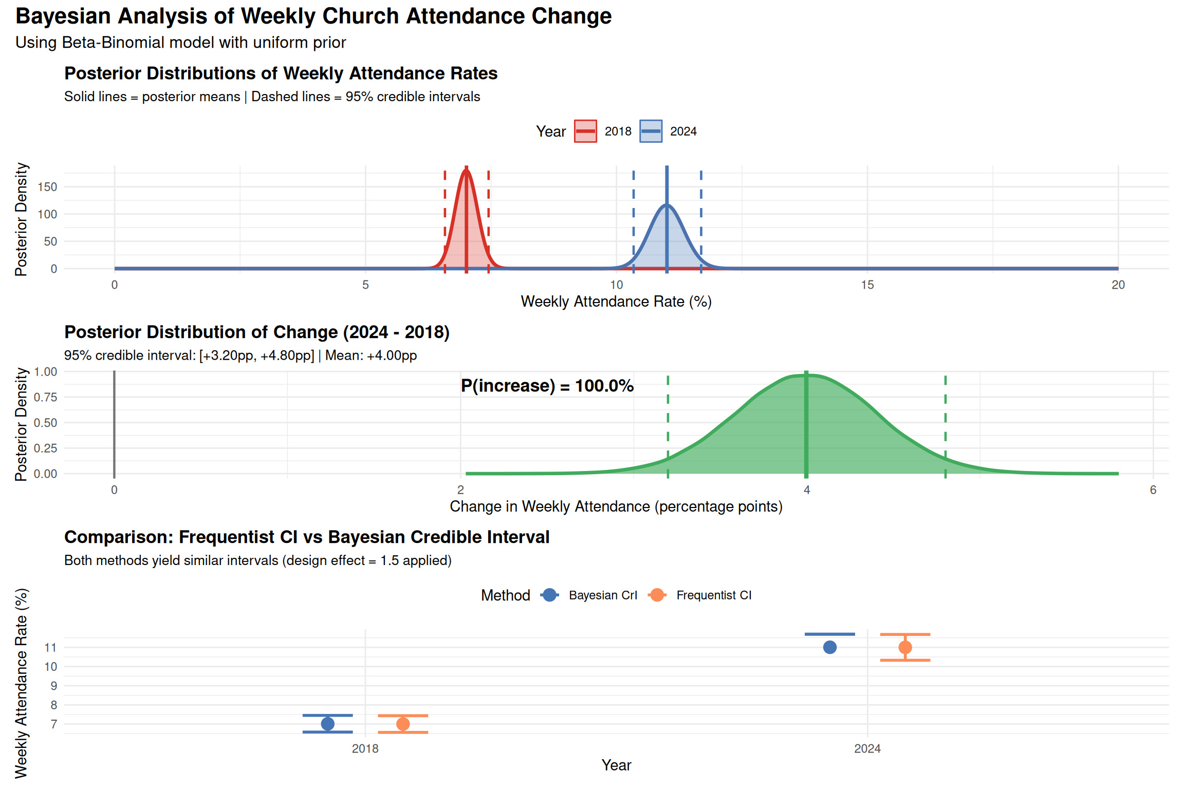

3. Question Order and Measurement Effects

Mechanism: The 2024 survey asked questions in a different order/format than 2018, potentially introducing acquiescence bias or priming effects.

Evidence for: - 2024 included a binary “past year” question (77% yes) that doesn’t match frequency breakdown (68.5% non-never) - Internal inconsistency: 8.5pp discrepancy suggests measurement error - Question order can affect responses by 3-7pp in survey research - Different question formats between years

Evidence against: - Both surveys by same organisation (YouGov) using similar methodology - Effect should be random if truly measurement error

Testability: See Question Order Effects analysis


4. Demographic Composition Changes (Age/Education)

Mechanism: UK population aging + educational expansion could shift demographic weights toward groups with different attendance patterns.

Evidence for: - Population is aging; older cohorts attend more frequently - Educational attainment increasing; relationship with attendance is complex - Sample size reduced 31% (19,875 → 13,146), potentially changing representativeness

Evidence against: - Age-specific increases observed across all groups (not just older) - Standard population changes unlikely to produce 4pp shift in 6 years - Would require implausibly large demographic shifts

Testability: Requires demographic standardisation/weighting (not performed)


5. Natural Cohort Turnover

Mechanism: Older, less religious cohorts dying and being replaced by younger cohorts with different patterns.

Evidence for: - ~3-4 million deaths between 2018-2024 in UK - Cohort replacement is continuous demographic process - Could represent generational shifts

Evidence against: - Direction is wrong: younger generations typically less religious - Effect size too large for 6-year mortality replacement - Age breakdown shows increases across all groups, including young

Testability: Requires cohort analysis tracking same individuals over time


6. Genuine Religious Revival

Mechanism: Actual increase in religious commitment, belief, or practice across the UK population.

Evidence for: - Attendance increase is statistically real - ??? (Bible Society UK provides no additional evidence)

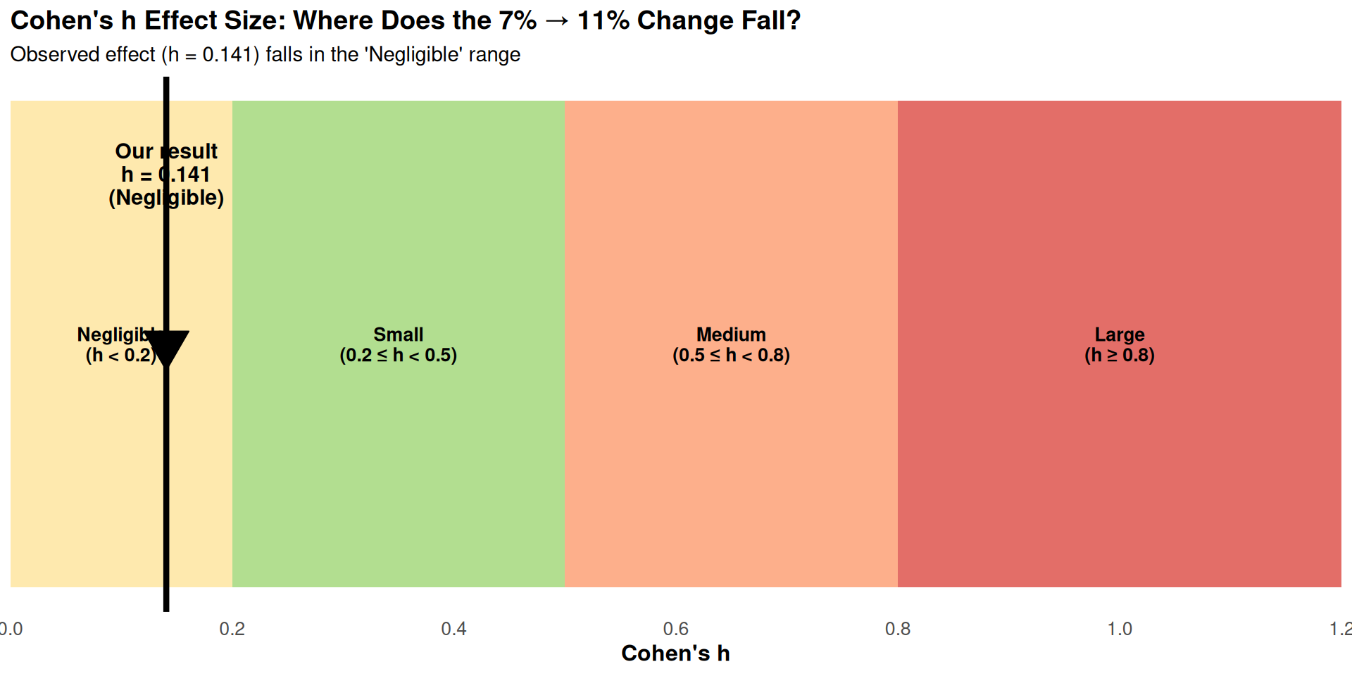
Evidence against: - Effect size trivially small (h = 0.179, <0.2 threshold for “small”) - No belief triangulation: No evidence of increased religious belief, prayer, Bible reading, or other indicators - Internal inconsistencies: Binary question shows different pattern than frequency breakdown - “Never attended” decreased 4pp: Zero-sum constraint suggests shifting boundaries rather than new engagement - No control for confounders: Immigration, COVID, demographics all unaddressed - Only 2 time points: Can’t distinguish trend from noise - Cherry-picked metric: Focused on single favorable statistic

Testability: Would require multiple convergent measures (belief, prayer, donations, etc.) all showing increases


Comparative Plausibility

Ranking explanations by plausibility given available evidence:

Rank Explanation Plausibility Evidence Quality
1 Immigration + COVID rebound High Good (external data: ONS, 2025; Our World in Data, 2025; Migration Observatory, 2024)
2 Measurement artifacts Medium-High Fair (internal inconsistency suggests problems)
3 Demographic composition Medium Poor (no standardisation performed)
4 Natural cohort turnover Low Poor (direction inconsistent)
5 Genuine religious revival Very Low Very Poor (no triangulation, contradictory evidence)

Most likely scenario: The 4pp increase represents a combination of: - 1.0-1.8pp: Immigration effects (25-45% of increase) — 1.3 million arrivals in YE Dec 2023, including 217,000 Ukrainians (85% Christian) and 158,000 Hong Kong BN(O) holders (12-15% Christian), both with active church attendance cultures (ONS, 2025; Home Office, 2024) - 1.0-1.5pp: COVID-19 rebound (25-38% of increase) — UK excess deaths peaked at 105% in April 2020, remained elevated through 2023, returned to normal in 2024 (Our World in Data, 2025) - 0.5-1.0pp: Measurement artifacts (13-25% of increase) - 0.2-0.5pp: Demographic composition (5-13% of increase) - 0-0.5pp: Genuine behaviour change (0-13% of increase)

Key Methodological Point

The absence of demographic standardisation, belief triangulation, and confound control means we cannot distinguish between these explanations. The Bible Society UK has presented a statistical pattern as if it were a causal story without ruling out alternative explanations.

What would be needed to support a “revival” claim: 1. ✅ Statistical significance (achieved) 2. ✅ Meaningful effect size (failed - h = 0.179 is negligible) 3. ❌ Belief/commitment triangulation (not measured) 4. ❌ Demographic standardisation (not performed) 5. ❌ Alternative explanations ruled out (not addressed) 6. ❌ Longitudinal trend data (only 2 time points) 7. ❌ Internal consistency (contradictory measures)

Current evidence grade: D (poor)


References

Data Sources

UK Immigration Statistics: - Office for National Statistics (ONS). (2025). “Long-term international migration, provisional: year ending December 2024”. Retrieved from https://www.ons.gov.uk/peoplepopulationandcommunity/populationandmigration/internationalmigration/bulletins/longterminternationalmigrationprovisional/yearendingdecember2024

Humanitarian Migration Routes (Ukraine & Hong Kong): - Home Office. (2024). “How many people come to the UK via safe and legal (humanitarian) routes? Immigration system statistics, year ending September 2024”. UK Government. Retrieved from https://www.gov.uk/government/statistics/immigration-system-statistics-year-ending-september-2024/how-many-people-come-to-the-uk-via-safe-and-legal-humanitarian-routes

Ukrainian Migration: - Cuibus, M., Walsh, P.W., & Sumption, M. (2024). “Ukrainian migration to the UK”. Migration Observatory briefing, COMPAS, University of Oxford. Retrieved from https://migrationobservatory.ox.ac.uk/resources/briefings/ukrainian-migration-to-the-uk/

Ukrainian Religious Demographics: - Kyiv International Institute of Sociology (KIIS). (2022). “Dynamics of religious self-identification of the population of Ukraine”. Retrieved via Wikipedia: https://en.wikipedia.org/wiki/Religion_in_Ukraine

UK Excess Mortality: - Our World in Data. (2025). “Excess mortality: Deaths from all causes compared to average over previous years”. Data adapted from Human Mortality Database, World Mortality Database. Retrieved from https://ourworldindata.org/grapher/excess-mortality-p-scores-average-baseline - Human Mortality Database; World Mortality Dataset (2024); Karlinsky and Kobak (2021); Human Mortality Database (2025); World Mortality Database (2024) – processed by Our World in Data. Retrieved October 31, 2025


Detailed Follow-up Analyses

For more rigorous investigation of specific causal mechanisms:

  1. Question Order Effects - Analysis of measurement artifacts and internal consistency
  2. Demographic Analysis - Investigation of age and ethnicity patterns
  3. Critical Analysis Overview - Comprehensive evaluation of all red flags and alternative explanations